Dynamic Relaxation Analysis

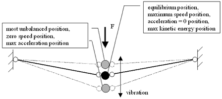
Dynamic relaxation is an analysis method for nonlinear statically loaded structures using a direct integration dynamic analysis technique. In dynamic relaxation analysis it is assumed that the loads are acting on the structure suddenly, therefore the structure is excited to vibrate around the equilibrium position and eventually come to rest on the equilibrium position. In order to simulate the vibration, mass and inertia are needed for each of the free nodes. In dynamic relaxation analysis, artificial mass and inertia are used which are constructed according to the nodal translational stiffness and rotational stiffness. If there is no damping applied to the structure, the oscillation of the structure will go forever, therefore, damping is required to allow the vibration to come to rest at equilibrium position. There are two types of damping: viscous damping and kinetic damping. Kinetic damping is an artificial damping which will reposition the nodes according to the change of system kinetic energy.

Damping

There are two types of viscous damping, the "actual" viscous damping and an "artificial" viscous damping. Viscous damping will apply the specified (or automatically selected) percentage of the critical damping to the system. Artificial viscous damping will artificially reduce the velocity at each cycle by the specified (or automatically selected) percentage of velocity in previous cycle. Once artificial viscous damping is used, kinetic damping will be disabled automatically. By applying one or both of these artificial damping methods, the vibration will gradually come to rest at the equilibrium position and this will be the solution given by dynamic-relaxation analysis.

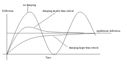
The structure below shows the effect of viscous damping on the dynamic relaxation analysis process. The oscillation of the structure eventually comes to rest at the static equilibrium position if viscous damping is applied. The problem with viscous damping is that it is not an easy task to estimate the critical damping of the structure.

Kinetic damping is unrelated to conventional concepts of damping used in structural dynamic analysis. It is an artificial control to reduce the magnitude of the vibration in order to make it come to rest. It is based on the behaviour of structures with only one degree of freedom or the vibration of a multiple degree of freedom structure in a single mode. For these cases it is known that the structure’s kinetic energy reaches a maximum at the static equilibrium position.

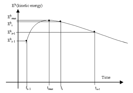
The structure’s kinetic energy is monitored in the analysis at each time increment. The Kinetic energy increases as the nodes approach equilibrium position and starts to decrease once the nodes are away from equilibrium position. Once the kinetic energy starts to decrease, an estimate of the equilibrium position of the nodes can be interpolated from the previous nodal positions and kinetic energies.

At this point the kinetic damping process is applied. The vibration is stopped and the nodes repositioned to correspond to the maximum kinetic energy. Assuming the relationship between structural kinetic energy and time is a parabolic, then the moment at which the kinetic energy peaked can be calculated. Based on the previous nodal displacements and rotations, the equilibrium positions of the nodes can be estimated. After shifting the nodes to their optimum positions, the analysis will restart again by resetting the time, speed, and acceleration to be zero.

Since it is unlikely that a multiple degree of freedom structure will vibrate in a single mode, it is impossible to find the equilibrium position just by reaching the maximum kinetic energy of the structure once or twice. Nevertheless, previous experience has shown that the use of kinetic damping is very efficient in searching for the equilibrium position in dynamic relaxation analysis.

Solution Process

The following steps are used in a dynamic relaxation analysis.

1. Compute equivalent nodal forces and moments. In this process, member loads are converted into nodal force or moments. These are the forces that initiate vibration.
2. Construct dummy mass and dummy inertia for the unrestrained (active) nodes according to the translational and rotational stiffness of the members at the nodes
3. Compute the acceleration, speed, and displacement for each node at each cycle.
4. Compute a new nodal position and rotation for each node at each cycle; update the nodal stiffness and member force acting on the nodes.
5. Check the force and moment residuals at each node at the current position.
6. If no residual exceeds the limit, the analysis is considered to have converged and the final position is considered as the equilibrium position of the structure.
7. If any residual is not satisfied, the analysis is continued to the next step.
8. Compute the total kinetic energy of the structure. If the kinetic energy at a cycle overshoots the maximum, it is considered that the equilibrium position has been passed. Therefore, all nodes will be re-positioned so that they are closer to the equilibrium position. Reset the speed and acceleration to be zero and let the structure start to vibrate again from the new position.
9. After analysis has been converged, the element forces, moments and stresses are calculated according to the final equilibrium position of the nodes.

Fictitious masses and inertia

To speed up and simplify dynamic relaxation analysis, fictitious (dummy) masses and inertia rather than real masses and inertia are used in dynamic relaxation analysis. The fictitious masses and inertia are generated automatically in the solver. However, fictitious masses and inertia can be adjusted pre and during analysis by applying dummy mass and inertia factors and/or dummy mass and inertia power.

The fictitious masses and inertias calculated by the program are designed to be small enough for convergence to be reasonably fast but large enough to prevent nodes shifting too much in one cycle, which causes the solution method to become unstable. To this end, it is logical to take the fictitious masses and inertia proportional to the nodal translational stiffness and rotational stiffness respectively. From previous experience, it is found that the best estimate of the fictitious masses and inertia are two times the nodal translational stiffness and rotational stiffness respectively and they are calculated as follows

• Fictitious mass of a node = 2 × sum of translational stiffness of the elements connected to the node
• Fictitious inertia of a node = 2 × sum of rotational stiffness of the elements connected to the node

Control parameters

The iterative dynamic relaxation process continues until convergence criteria (unbalanced nodal force and moment) are met. If this does not happen, the iteration will continue for a maximum number of cycles, or analysis time in minutes.

It is almost impossible to achieve 100% accurate results in nonlinear analysis, so an acceptable residual (tolerance) force and moment should be specified. The residual may be absolute or relative.

If relative residual is selected, the actual force residual and moment residual at each node are calculated from

$$\begin{aligned}\Delta f &= \rho_{f}\frac{\sum{f}}{n} \\ \Delta m &= \rho_{m}\frac{\sum{m}}{n}\end{aligned}$$

where

$\Delta f,\Delta m$ are force residual and moment residual respectively

$\rho_{f},\rho_{m}$ are relative force residual and relative moment residual respectively

$\sum f$ is the sum of the total imposed loads including both nodal and member loads

$n$ is the number of nodes in the structure

If there is no imposed load, e.g. a structure subjected only to support settlement, the force residual and moment residual are calculated from

$$\begin{aligned}\Delta f &= 0.01 \times \rho_{f}\frac{\sum_{}^{}K_{f}}{n}\\ \Delta m &= 0.01 \times \rho_{m}\frac{\sum_{}^{}K_{m}}{n}\end{aligned}$$

where

$\sum K_{f},\sum K_{m}$ are the sum of nodal translational stiffness and rotational stiffness of all the nodes in the structure.

If an absolute residual is selected, the specified force residual and moment residual will be used in the analysis.

Beam – Axial force

The axial force $f_{x}$ of a beam is first calculated as

$$f_{x} = f_{p} + EA\varepsilon$$

where $f_{p}$ is the pre-stress force.

If this force is greater than the yield capacity in tension it is set to the yield capacity in tension; if it is less than the yield capacity in compression it is set to the yield capacity in compression. The yield capacities are

$$f_{y,tens} = A\sigma_{y,tens}$$ $$f_{y,comp} = A\sigma_{y,comp}$$

where $\sigma_{y,tens}$ is the tensile yield stress and $\sigma_{y,comp}$ is the compressive yield stress

The strain is calculated as

$$\varepsilon = \frac{\left( u_{2x} - u_{1x} \right) - l}{l}$$

Where $l$ is the initial length as defined by the node positions (or the ‘initial length’ as specified by the user) modified for temperature.

Beam – Shear force and torsion

The shear modulus of a beam is assumed to be

$$G = \frac{E}{2(1 + \nu)}$$

The shear strain caused by a shear force is considered to be uniform over the whole beam for planes normal to a principal axis. The shear strain between a principal axis and the local beam x axis is taken as

$$\varepsilon_{xy} = \frac{\sigma_{xy}}{G}, \varepsilon_{xz} = \frac{\sigma_{xz}}{G}$$

and the effective shear stress is taken as

$$\sigma_{xy} = \frac{V}{k_{y}A} \sigma_{xz} = \frac{V}{k_{z}A}$$

Where $k_{y}$ $k_{z}$ are the shear factor along the principal axis closest to the local beam y/z axis.

The angle by which a beam is twisted about its local x axis is simply considered to be

$$\frac{M_{x}l}{GJ}$$

Beam – Axial force – flexural stiffness interaction

If slenderness effects are to be considered the bending stiffness of a beam is modified according to the axial load by using Livesey’s ‘stability functions’[^1].

For a continuous/continuous beam within the elastic range the bending moment at end 1 is taken as

$$M_{1} = \frac{EI\left( S \times \theta_{1} + SC \times \theta_{2} \right)}{l} \tag{Equation A}$$

$S$ and $SC$ are derived from series

$$S = \frac{\left( \frac{2}{3!} - \frac{4}{5!}k + \frac{6}{7!}k^{2} - \frac{8}{9!}k^{3} + \cdots \right)}{\left( \frac{2}{4!} - \frac{4}{6!}k + \frac{6}{8!}k^{2} - \frac{8}{10!}k^{3} + \cdots \right)}$$ $$SC = \frac{\left( \frac{1}{3!} - \frac{k}{5!} + \frac{k^{2}}{7!} - \frac{k^{3}}{9!} + \cdots \right)}{\left( \frac{2}{4!} - \frac{4}{6!}k + \frac{6}{8!}k^{2} - \frac{8}{10!}k^{3} + \cdots \right)}$$

where

$$k = \frac{f_{x} \times l^{2}}{EI}$$

and compression is positive.

For a continuous/pinned beam within the elastic range the bending moment at end 1 is taken as

$$M_{1} = \frac{EI\left( S^{''} \times \theta_{1} \right)}{l} + C \times M_{2} \tag{Equation B}$$

$S^{''}$ and $C$ are derived from series

$$S^{''} = \frac{\left( 1 - \frac{k}{3!} + \frac{k^{2}}{5!} - \frac{k^{3}}{7!} + \cdots \right)}{\left( \frac{2}{3!} - \frac{4}{5!}k + \frac{6}{7!}k^{2} - \frac{8}{9!}k^{3} + \cdots \right)}$$ $$C = \frac{\left( \frac{1}{3!} - \frac{k}{5!} + \frac{k^{2}}{7!} - \frac{k^{3}}{9!} + \cdots \right)}{\left( \frac{2}{3!} - \frac{4}{5!}k + \frac{6}{7!}k^{2} - \frac{8}{9!}k^{3} + \cdots \right)}$$

where $M_{2}$ is the moment at end 2 and compression is positive.

These series are used to pre-calculate $S$, $SC$, $S^{''}$ and $C$ for ten values of $K$. During calculation cycles values of $S$, $SC$, $S^{''}$ and $C$ are interpolated for the current value of $K$.

Beam – Yielding

For an explicitly defined section the bending moments about the principal axes are limited to the following value

$$0.45 \times \left( \sigma_{y,tens} - \sigma_{y,comp} \right) \times \sqrt{A \times I_{p}}$$

For equal yield stresses this is a good approximation to the plastic bending moment capacity.

The axial force is computed as above.

The calculations for the axial force and for the bending moments about the principal axes are all performed independently. Beams are assumed to behave elastically up to the limiting force or bending moment. Thus plastic behaviour is only modelled with any degree of realism for cases where either

• only axial forces are significant or
• only bending about one principal axis is significant, the tensile and compressive yield stresses are similar and the transition between first yield and full plasticity can be ignored.

If the bending moment at one end of a beam has been limited to the plastic moment capacity, the bending moment at the other end is obtained by using equation B above

$$M = \frac{EI \times S^{''} \times \theta}{l} + C \times M_{plas}$$

This bending moment is in turn limited to the plastic moment capacity.

For a beam with a standard shape section and a specified yield stress, the program calculates the tensile and compressive yield forces of the section, which are taken to be

$$f_{y,tens} = A\sigma_{y,tens}$$ $$f_{y,comp} = A\sigma_{y,comp}$$

The program then constructs a ‘look up’ table for each shape before the commencement of calculation cycles.

The ‘look up’ table contains values of

• bending moment causing first yield (i.e. the lowest bending moment at which with elastic behaviour yield stress is attained in tension or compression at one point in the section)
• plastic bending moment (i.e. the bending moment with the section on one side of the neutral axis at the tensile yield stress and on the other side of the neutral axis at compressive yield stress).

for

• nine values of axial force equally spaced between the tensile and compressive yield axial loads of the section.
• angles of applied moment at intervals of 15 degrees from 0 to 345 degrees with reference to the principal axis that is nearest to the beam local y axis.

During calculation cycles the program computes the bending moment at first yield and the plastic bending moment in a beam for the current axial force and angle of applied bending moment by linear interpolation between the values in the “look up” table (both bending moments are of course zero when the axial force equals the tensile or compressive yield force, and the axial force of a beam is limited to values between the tensile and compressive yield forces)

The program initially calculates the forces and bending moments at each end of a beam assuming elastic behaviour. If the net bending moment at the first end is greater than the moment causing first yield then the bending moment is modified according to the formula

$$M_{i + 1} = M_{y} + 0.5\left( M_{i} - M_{y} \right)\tag{Equation C}$$

If the bending moment at the first end of a beam is modified, the bending moment at the second end is obtained by using equation B

$$M_{2} = \frac{EI \times S^{''}\theta}{l} + C \times M_{1,mod}$$

If the bending moment at the second end exceeds that at first yield, it is modified in the same way as was the one at the first end, and the bending moment at the first end is obtained by using equation B

$$M_{1} = \frac{EI \times S^{''}\theta}{l} + C \times M_{2,mod}$$

If this bending moment is greater than the moment causing first yield, the whole process is repeated until the bending moments cease to be modified.

Equation C is equivalent to halving the stiffness of a beam at first yield.

Fabric- Stress computation

The warp and weft directions are assumed to be perpendicular. The direct and shear strains are first computed for the warp and weft directions assuming uniform strains over each triangle and the stresses are calculated from the equations

$$\sigma_{xx} = \frac{E_{xx}\varepsilon_{xx} + E_{yy}\nu_{yx}\varepsilon_{yy}}{1 - \nu_{xy}\nu_{yx}}\tag{A}$$ $$\sigma_{yy} = \frac{E_{yy}\varepsilon_{yy} + E_{xx}\nu_{xy}\varepsilon_{xx}}{1 - \nu_{xy}\nu_{yx}}\tag{B}$$ $$\sigma_{xy} = G\varepsilon_{xy}$$

where $x$ is the warp direction and $y$ is the weft direction.

The principal stresses are then computed. If a triangle is set to take no compression, compressive principal stresses are set to zero.

The forces exerted by the triangle are calculated from the principal stresses.

Equations A and B are obtained by rewriting

$$\varepsilon_{xx} = \frac{\sigma_{xx} - \nu_{yx}\sigma_{yy}}{E_{xx}}$$

and

$$\varepsilon_{yy} = \frac{\sigma_{yy} - \nu_{xy}\sigma_{xx}}{E_{yy}}$$

Poisson’s ratio for pure warp stress $\nu_{xy}$ is defined in the material table. $\nu_{yx}$, the Poisson’s ratio for pure weft stress is calculated from

$$\nu_{yx} = \frac{E_{xx}\nu_{yx}}{E_{yy}}$$

If no shear modulus is specified it is calculated as

$$G = \frac{0.5\left( E_{xx} + E_{yy} \right)}{2\left( 1 + 0.5\left( \nu_{xy} + \nu_{yx} \right) \right)}$$

For isotropic materials where $E_{xx} = E_{yy} = E$ and $\nu_{xy} = \nu_{yx} = \nu$ this is equivalent to

$$G = \frac{E}{2(1 + \nu)}$$

This corresponds to elastic behaviour.